This notes is for the book - High performance java persistence

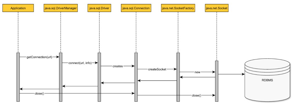
The JDBC API provides common interface for communicating to the db server. To communicate to a db server, a Java program must first obtain a java.sql.connection.. java.sql.Driver is the actual db connection provider. java.sql.DriverManager provides the more convenience since it can also resolve the JDBC driver associated with the current db connection URL.

DriverManager

Every time the getConnection() method is called, the driver manager will request a new physical connection from the underlying driver.

In a two-tier architecture, the application is run by single user and each instance uses a dedicated db connection. Each database server, based on the underlying resources can only offer a limited number of connections.

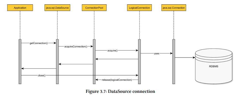
DataSource

Intermediate data layer

In a three-tier architecture, the middle tier acts as a bridge between user requests and various data sources (relation databases, messaging queues).

Having this intermediate layer has numerous advantages. It acts as a db connection buffer that can mitigate user request traffic spikes by increasing request response time, without depleting db connections or discarding incoming traffic. The application server provides only logical connections (proxies or handles), so it can intercept and register how the client API interacts with the connection object.

A three-tier architecture can accommodate multiple data sources or messaging queue implementations. To span a single transaction over multiple sources of data, a distribution transaction manager becomes mandatory. In Java Transaction API (JTA), the transaction manager must be aware of the logical connections the client has acquired as it has to commit or roll them back according to the global transaction outcome.

By providing logical connections, the application server can decorate the db connection handles with JTA transaction semantics.

java.sql.DriverManager - is a physical connection factory.
java.sql.DataSource - is a logical connection provider interface.

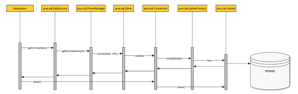
1. Application data layer asks the DataSource for a db connection.
2. The DataSource will use the underlying driver to open a physical connection.
3. A physical connection is created, and TCP socket is opened.
4. The DataSource doesn’t wrap the physical connection and simply lends it to the application layer.
5. The application executes statements using acquired db connection.
6. When the connection is no longer needed, the application closes the physical connection along with the underlying TCP socket.

When using a connection pooling solution, the connection acquisition time is between two and four orders of magnitude smaller.

Why is pooling much faster?

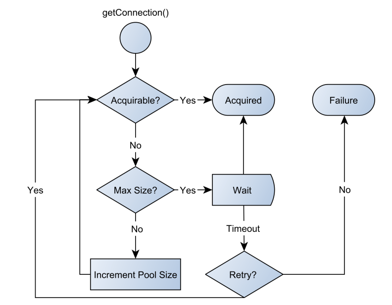
1. When a connection is being requested, the pool looks for unallocated connections.
2. If the pool finds a free one, it handles it to the client.
3. If there is no free connection, the pool tries to grow to its maximum allowed size.
4. If the pool already reached its maximum size, it will retry several times before giving up with a connection acquisition failure exception.
5. When the client closes the logical connection, the connection is released and returns to the pool without closing the underlying physical connection.

Most connection pooling exposes a DataSource implementation that either wraps an actual database specific DataSource or the underlying DriverManager utility.

1. The connection pool offers a proxy or a handle instead of a physical connection to the client.

2. When the connection is in use, the pool changes its state to allocated. (To prevent two concurrent threads from using the same db connection).

3. The proxy intercepts the connection close method call, it notifies the pool to change the connection state to unallocated.

   Connection pool can act as a bounded buffer for the incoming connection requests. If there is a traffic spike, the connection pool will level it, instead of saturating all the available db resources.

   Configuring the right pool size is not a trivial thing to do. Provisioning the connection pool requires understanding

   1. Application-specific database access patterns
   2. Connection usage monitoring

Whenever the number of incoming requests surpass the available handlers, there are two options to avoid system overloading.

1. Discarding the overflowing traffic (affects availability)
2. Queuing requests and wait for busy resources to be available (increasing response time)

Discarding the surplus traffic is usually a last resort measure. Most connection pooling solutions first attempt to enqueue overflowing incoming requests. By putting an upper bound on the connection request wait time, the queue is prevented from growing indefinitely and saturating the application server resources.

For a given incoming request rate, the relation between queue size and average enqueuing time is given by one of the most fundamental laws of queuing theory.

Queuing theory capacity planning

Little’s Law

Little Law is a general purpose equation applicable to a queuing system that is in a stable state.

Assuming that the application-level transaction uses the same db connection through its life-cycle,

• If the average transaction response time is 100 milliseconds (0.1 seconds).
• If the average connection acquisition rate is 50 requests per second.

The average number of connection requests in the system is 50 * 0.1 = 5 connection requests. (Both the requests being serviced and the ones waiting in the queue).

A pool size of 5 can accommodate the average incoming traffic without having to enqueue any connection requests.
If the pool size is set to 3, then on average 2 requests are enqueued and waiting for connections to be available.

Queuing theory

• If the average service time is 100 milliseconds (0.1 seconds).
• If the average connection acquisition rate is 50 requests per second.
  We concluded that the pool can offer at most 5 connections (there are at most 5 in-service requests).

In queuing theory, throughput is represented by the departure rate (μ), for a connection pool, it represents the number of connections offered in a given unit of time:

If the arrival rate outgrows the connection pool throughput, the overflowing requests must wait for connections to become available.

A one second traffic burst of 150 records is handled as

• The first 50 requests can be served in the first second.
• The following 100 requests are first enqueued and processed in the following two seconds.

For a constant throughput, the number of enqueued connection requests is proportional to the connection acquisition time.

The total time required to process the spike is given by the formula:

Assuming there is a traffic spike of 250 requests per second for 3 seconds. Then the Lspike is 750 requests. If the throughput (μ) is 50 requests / second, Then the total time to process all the records is 15 seconds.

A real-life connection pool monitoring example

The dynamics of enterprise systems are difficult to express with equations like Queuing theory and metrics become fundamental for resource provisioning. By continuously monitoring the connection usage patterns, it is much easier to react and adjust the pool size when initial configurations doesn’t hold anymore.

In case of an unforeseen traffic spike, the connection acquisition time could reach the DatasSource timeout threshold.

Following were the observations made while conducting an experiment using an opensource connection pool and batch processor.